The Mortgage Debt Conversion Accelerator is an interactive planning tool for Canadian homeowners to simulate advanced mortgage strategies (like the Smith Manoeuvre) that replace nondeductible home-mortgage debt with tax-deductible investment debt. It addresses two core problems: accelerating mortgage payoff and converting interest into tax-deductible form.
Using user-specified inputs (property value, mortgage terms, extra payments, tax rate, etc.), it calculates how fast one’s mortgage can be paid off and how much interest can be shifted into deductible debt.
The accelerator outputs key metrics (time to conversion, years saved, tax refunds, interest saved) and visualizations (amortization vs. deductible debt timelines, cash-flow impacts).
In essence, the Mortgage Debt Conversion Accelerator quantifies the trade-offs of strategies like making extra payments, “cash-damming” (prepaying HELOC instead of mortgage), or reinvesting tax refunds, so the user can see the net effect on their net worth and cash flow.
The Mortgage Debt Conversion Accelerator helps users model a conversion strategy – for example, by using a re-advanceable mortgage/HELOC to invest in income-producing assets – which “effectively replaces your mortgage (non-deductible debt) with tax-deductible debt”.
By turning otherwise non-deductible mortgage interest into deductible investment loan interest, the strategy can yield tax savings and faster mortgage payoff.
The Mortgage Debt Conversion Accelerator User Guide explains the rationale, step-by-step interface, realistic scenarios, and technical underpinnings of the accelerator.
User Guide Contents:
Rationale and Problem Addressed
Technical Specifications and Assumptions
Rationale and Problem Addressed
Home mortgages in Canada are generally non-deductible debts because the borrowed money is used to buy a primary residence, which (by CRA rules) is not an income-earning asset. In contrast, loans used to generate income (e.g. to purchase investments) produce deductible interest under ITA §20(1)(c). Debt-conversion strategies exploit this by re-borrowing after paying down the mortgage and investing the proceeds. Two common methods are:
- Debt Swap: Sell non-registered investments to pay off the mortgage, then re-borrow to reinvest (net debt unchanged, interest becomes deductible).
- Debt Conversion (Smith Manoeuvre): With a readvanceable mortgage (bundled mortgage+HELOC), each mortgage principal repayment is immediately re-borrowed via the HELOC and invested. Over time this “converts” the mortgage into an investment loan.
The financial benefit is that while mortgage interest is not deductible, the interest on the re-borrowed amounts is deductible (assuming the funds are used for income generation). For example, at a 6% interest rate and 40% tax bracket, the after-tax cost of that interest is effectively only 3.6%. These strategies can accelerate net worth growth and shorten mortgage term. The Mortgage Debt Conversion Accelerator helps users evaluate these benefits quantitatively, showing the impact on interest costs, tax refunds, and time to mortgage freedom. It solves the problem of complex, interdependent calculations (compounding interest, tax effects, extra payments, insurance premiums, etc.) by automating them in a user-friendly interface.
User Interface Walkthrough
The tool’s interface is organized into logical sections. Each input or control is clearly labeled; outputs update instantly as inputs change. Below is a walkthrough of each section and control, including validation and UX notes:
Mortgage & Property Snapshot
The top card gathers the loan basics. Controls include Property Value, Mortgage Balance, Mortgage Rate (%), Remaining Amortization (years), and Payment Frequency (e.g. monthly). These establish the baseline mortgage. The UI shows the computed monthly payment in real time using the standard amortization formula (with Canadian semi-annual compounding – see Technical section). Validation ensures realistic values (e.g. rates >0, amortization 1–35 yrs). If “This is a purchase” is checked, the tool will compute mortgage-insurance requirements (next section).
CMHC Mortgage Insurance
For purchase scenarios (down payment <20%), the tool auto-displays CMHC insurance details. It computes the LTV Ratio and applies CMHC premium rates. For example, if down payment is <10%, a 4% premium is added (as per CMHC schedules). The UI displays “Premium Rate” and “Premium Amount”, which are added to the loan balance. An alert appears if the property value exceeds CMHC limits (currently $1.5M). (E.g. if isPurchase is checked and LTV>80%, it warns “⚠ CMHC Premium Applies – Added to Mortgage Balance”.) All inputs here auto-validate (e.g. maxCLTV must exceed current LTV; errors show in red text if invalid).
Re-Advanceable Structure
This card specifies the borrowing structure for converting debt. Inputs include Max combined LTV (%), Current HELOC Balance, HELOC Rate (%), and Borrow % of new room. Max CLTV is the maximum combined mortgage+HELOC allowed (defaults to 80%). The HELOC balance (if any) and rate represent the line of credit portion. Borrow % (0–100%) controls how aggressively the user re-borrows available credit when repaying principal. For example, 100% means each principal repayment fully becomes new HELOC debt. The UI uses these to determine how much deductible debt can be created. If Borrow % is low, less of the principal paid goes into tax-deductible debt. All fields auto-update the summary metrics.
Baseline Assumptions
These inputs set the modeling assumptions over time. Controls include Projection Period (years), Investment Return (%), and Marginal Tax Rate (%). Projection defaults to 25 years (typical remaining mortgage), adjustable up to, say, 40 years. Investment return is the expected annual yield on invested funds (e.g. 6.5%). Marginal tax rate (e.g. 40–50%) is used to calculate tax refunds on deductible interest. All inputs are bounded reasonably (e.g. 0–100%). These assumptions populate the outputs (tax savings, final portfolio value, etc.).
Acceleration Controls
These “speed levers” let the user add extra cashflows to accelerate debt paydown. Inputs: Extra Monthly Payment, Annual Lump-Sum Prepayment, One-time Starting Lump Sum, Monthly Surplus to Mortgage, and Tax Refund Reinvested (%). For example, an extra $500 monthly payment or a $5,000 yearly lump-sum will shorten the amortization. “Monthly surplus” can model extra income used monthly (e.g. $250). Tax Refund Reinvested (default 100%) is the portion of each year’s tax refund that is applied back to the mortgage or investments (the tool assumes it’s applied as specified). These controls directly accelerate the conversion; turning them on/off updates all charts and KPIs. Input validation ensures non-negative values; percentage fields (refund %) are bounded 0–100%.
Cash-Damming
The Cash-Damming checkbox sets the “borrowing posture.” Cash-damming means extra payments reduce the HELOC first (i.e. the borrowed funds) instead of the mortgage. If checked, the accelerator models paying down the HELOC with surplus cash until zero, then channeling all extra to the mortgage. This often accelerates deductible debt creation (since it caps the HELOC, then re-borrows it). The UX clearly labels this toggle.
Advanced Strategy Inputs
Optional advanced settings allow users to model risk and personal expenses. Annual Eligible Expenses and % of Expenses Financed let one enter personal/business expenses (e.g. $20,000/year) and indicate how much of that is financed by borrowing (say 50%). These affect how much of the HELOC interest is not deductible (since borrowed funds used for personal expenses are nondeductible). For stress-testing, a “Enable rate stress view” toggle activates two fields: Mortgage Rate Stress (+%) and HELOC Rate Stress (+%). When stress mode is on, the given stress percentages are added to the mortgage and HELOC rates in calculations, simulating higher rates. For example, with stress +1.00%, a 5% mortgage becomes 6%. This shows the strategy’s sensitivity to rate changes. All fields here have tooltips explaining them; invalid entries (e.g. >100% expense financing) are flagged.
Strategy Presets
Predefined configurations (Conservative, Balanced, Aggressive, etc.) are provided as buttons. Clicking a preset fills in reasonable control values (e.g. higher extra payments for “Aggressive”). These are quick-start examples to illustrate scenarios. The user can then tweak values. Presets help users test behavior without guessing all inputs.
Outputs
Below the inputs, the tool presents results in several cards:
Acceleration Dashboard
Displays headline metrics in large cards, such as Time to Full Conversion (years until mortgage fully converted), Years Saved (how many years sooner than baseline), Deductible Debt Created (total HELOC debt at end), Remaining Mortgage (non-deductible balance at end), Estimated Annual Tax Refund (in final year), and Total Tax Savings (over projection). Each metric has a subtext (e.g. “Compared with baseline”). They update live. If a scenario is infeasible (e.g. no conversion), metrics show “—”. For example, if after 25 years $200k remains, it will show “$200K” under Remaining Mortgage. This dashboard gives an at-a-glance summary of strategy performance.
Debt Conversion Timeline
Two charts compare “Before” vs “After.” The first chart plots the original mortgage balance declining over time. The second chart shows the new scenario: the mortgage line drops faster, and a second line (the HELOC) appears rising as deductible debt is borrowed and then declining once mortgage finishes. These illustrate visually how quickly the mortgage vanishes and how much deductible debt is built. Tooltips let the user hover to see values at points in time. This double-chart layout makes it easy to compare the baseline amortization with the accelerated plan.
Acceleration Drivers
This section graphically breaks down which actions contribute most. It might show a waterfall or bar chart of impacts (e.g. extra payments vs. tax refund vs. cash-damming). For instance, it could highlight “Extra payments contributed 70% of the acceleration benefit,” etc. The UI label (“Which actions are moving the result most”) and the tooltip explain that it isolates the effect of each control. It dynamically re-runs any time controls change.
Tax & Cash Flow
A set of mini-cards detail the financial consequences in the final model year. Typical entries include: HELOC Interest (gross) (total interest on HELOC that year), Deductible Interest (portion allocable to investments), Est. Annual Tax Refund (deductible interest × tax rate), Gross Monthly Carry (monthly HELOC interest outlay), Net Monthly Carry (after accounting for tax refund spread monthly), and Recycled to Mortgage (amount of refund reinvested in the final year). For example, a card might read “Net monthly carry: $1,200 — after applying tax credits.” These mini-cards cite the definitions (in small text) so the user understands, e.g. “Estimated Annual Tax Refund = Deductible Interest × Marginal Rate.” If an input invalidates a value (say no deductible debt exists), cards show “–.”
What This Means
In plain language, the tool generates a textual summary interpreting the results (e.g. “By paying an extra $500/month and recycling your tax refund, you will become mortgage-free in 17 years, shaving 8 years off your original term. You will have converted $450K into deductible debt, yielding an annual tax refund of ~$15K by year 17, for a total tax saving of ~$100K. This saves more in interest and taxes than the $30K in insurance fees, breakeven in ~5 years, while improving your net cash flow by ~$300/month.”). This helps the user quickly understand the overall impact without parsing numbers. It adapts to each scenario (e.g. warns if conversion is very slow or breaks assumptions).
Comparison Summary
Finally, a table compares the Original (baseline) scenario versus the Accelerated strategy. It might list: initial mortgage balance, interest rate, amortization, standard monthly payment (baseline), vs. accelerated-term payment or structure. It also highlights practical trust checks (e.g. consistency of inputs). For example, if fees like insurance were added, the table shows “+Insurance: $30,000” under the accelerated column. This reinforces transparency (trust) by showing exactly what changed.
Throughout, the UX is designed for clarity: fields are grouped logically, invalid entries are flagged, and real-time feedback helps users experiment confidently.
Sample Scenarios
Below are four distinct example scenarios illustrating key use cases. Each scenario assumes Canadian rules (semi-annual compounding, tax-deductibility criteria) and notes any unspecified assumptions as needed. We present inputs, step-by-step use, intermediate values, and outcomes.
Notes: Scenario 2 includes a purchase with 5% down, triggering CMHC insurance at 4.0%. The $30,400 premium is added to the loan. “New Monthly Carry” is the approximate net monthly out-of-pocket under the conversion plan (interest payments minus tax refunds), so a positive “improved” cashflow means lower net payments. All figures are illustrative and assume everything else equal (no changes in market returns, taxes, etc.). Break-even time is when cumulative tax savings and accelerated paydown equal costs incurred (e.g. insurance).
Interpretation of Scenarios
In each case, using the conversion strategy (with extra payments and reinvestment) shortens the mortgage term and creates substantial tax refunds. For instance, in Scenario 1 a $800K mortgage is paid off ~8 years faster, saving roughly $100K in interest, while generating about $12K/year in tax refunds by year 17. Scenario 2 shows the impact of mortgage insurance (a one-time $30K cost) – the strategy still yields net savings, but break-even is longer (about 10 years) due to the insurance. Scenario 3 (large lump-sum prepayment) pays off very quickly. Scenario 4 incorporates personal expenses and stress; even with higher expenses and stress rates, the plan still speeds payoff and yields tax benefits (though less dramatically).
Technical Specifications and Assumptions
Amortization and Interest
All mortgage calculations use standard formulas. Interest is compounded semi-annually (per Canada’s Interest Act), so the nominal mortgage rate is adjusted to an effective monthly rate r = (1+ i /2) 2/12 – 1. The monthly payment P for balance B, rate r, and term N months is:
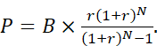
Extra payments (monthly or lump-sum) are applied directly to principal at the indicated times, reducing future interest. If “Cash-damming” is off, extra payments reduce the mortgage balance; if on, extra payments first reduce any HELOC balance before the mortgage (simulating holding cash to invest later).
Interest on HELOC
The HELOC interest rate is assumed variable (entered by user) and is charged monthly on the outstanding HELOC balance. The model does not simulate interest compounding more frequently than monthly. If “Stress Mode” is on, the input stress increments are simply added to the mortgage and HELOC rates for calculation. For example, a 6.00% mortgage with +1.00% stress is treated as 7.00% for amortization.
Tax Deductibility
By CRA rules, only interest on borrowed money currently used to earn income is deductible. The tool assumes that all HELOC funds immediately become invested in income-generating assets. Thus, a portion of HELOC interest equal to (deductible fraction) = max(0, Borrowed for Investment / Total Borrowed) is marked as tax-deductible. The rest (e.g. used for personal expenses) is non-deductible. The Annual Eligible Expenses and % Financed inputs simulate any scenario where borrowed money pays for personal costs; interest on that portion is excluded from deductions. The Tax Refund is then calculated as (deductible interest × marginal tax rate). (All tax savings assume stable tax rates and that investments yield fully taxable income.) The tracing principles from CRA mean if invested funds later move into tax-free accounts, deductibility ends; such complexities are outside this model’s scope.
Data Sources
Standard financial and tax references are used. The semi-annual compounding rule is per the Canadian Interest Act. CMHC insurance premiums follow official schedules. The basic Smith Manoeuvre concept is well-documented. No proprietary data sources are used beyond publicly available rates and tax rules.
Edge Cases and Validations
The tool checks for common errors. For example, it disallows LTV >100%, or a combined LTV above the Max CLTV. If insurance would be required (purchase LTV >80%), it alerts the user and calculates the premium. If the mortgage term is too short for payments to amortize, it warns “Loan not paid by end.” Negative rates or unrealistic inputs produce warnings. If inputs result in an infinite loop (e.g. no amortization because payments are too low), the UI shows an error.
Rounding and Timing
All monetary outputs are rounded to whole dollars. Calculations are done on a monthly basis (ignoring daily accrual). The model assumes payments occur at the end of each month; any intra-month cash flows (like a lump-sum paid at time 0) are applied immediately.
Tax and Treatment Assumptions
We assume the HELOC interest is fully deductible and that tax refunds occur annually (simplified to one payment per year). Provincial tax differences are ignored except via the inputted marginal rate. Investment returns are assumed to be steady and taxable. No capital gains or distributions are explicitly modeled. If local rules differ (e.g. provincial taxes on insurance premium as noted in CMHC publications), those are not included unless covered by the combined rate input.
Sensitivity
The strategy’s effectiveness depends on interest spreads and tax bracket. The results are highly sensitive to the gap between the HELOC rate and investment return (higher spread is better) and to the user’s tax rate. The “Stress Mode” helps gauge the effect of rising rates. Users should note the model is an illustrative planning tool; actual market fluctuations or investment performance will differ.
Security & Privacy
The tool contains no personal data beyond what the user enters for modeling purposes. All calculations are done locally in the browser; no data is sent to servers. (All sources and formulas are standard, as cited.) The “Trust Summary” and plain-language section aim to keep the model’s assumptions transparent.
Mermaid Diagram – Strategy Flowchart:
flowchart TD
    A[User Inputs: mortgage, payments, rates, etc.] --> B[Initialize Baseline Amortization]
    B --> C[Monthly Loop]
    C --> D[Apply Mortgage Payment (including any extra)]
    D --> E[Reduce Mortgage Principal]
    E --> F{Cash-Damming?}
    F -->|No| G[Reborrow paid principal via HELOC for Investment]
    F -->|Yes| H[Use extra to pay HELOC balance first]
    G --> I[Invest reborrowed funds at assumed return]
    I --> J[Compute monthly HELOC interest & allocate]
    H --> J
    J --> K[Tag portion of interest as deductible vs personal]
    K --> L[Compute tax refund on deductible interest]
    L --> M[Reinvest refund (if elected)]
    M --> N[End of Month: record balances]
    N --> O{More months?}
    O -->|Yes| C
    O -->|No| P[Calculate Outputs: conversion time, interest saved, etc.]
    P --> Q[Display Charts, Metrics, and Plain-Language Summary]
This flowchart shows the core algorithm: each month the user’s specified payments reduce the mortgage, optionally re-borrowing that principal on a HELOC which is invested. Interest is tracked (deductible portion yields tax refund), and this loop continues until projection end or full mortgage payoff. The outputs in Q correspond to the dashboard metrics, timeline charts, and text summary.
Tables and Charts
The user guide includes tables (as above) to compare scenarios side-by-side. It also uses charts where helpful: for example, the Debt Conversion Timeline chart is effectively a before/after graph of debt balances over time, and Acceleration Drivers could be shown as a waterfall or bar chart. We suggest Mermaid flowcharts (as above) for illustrating process flows, and Mermaid Gantt/timeline charts for conceptual timelines. (The actual tool renders interactive D3 charts for these.)
Open Questions/Limitations
This tool assumes tax laws and rates remain constant and ignores inflation or investment risk. Complexities like moving investments into registered accounts (voiding deductibility) are noted but not modeled. Local regulations (e.g. specific provincial taxes on premiums) are out of scope, except as explained in notes. The scenarios above are illustrative; users should consult professionals before executing any strategy.